Getting started with specsr-roman

Roman’s grism will deliver spectra at R ≈ 461, where the diagnostic complexes stay blended: Hα+[N II], [O III]+Hβ. specsr-roman super-resolves them with a three-stage network — and, more importantly, is calibrated so that lines the data could not have revealed are not drawn.

This notebook takes you from a fresh install to the numbers in the README:

1. download a small held-out subset of the training data,

2. load the published checkpoints,

3. super-resolve one spectrum and read what comes back,

4. see why the redshift is a PDF rather than a number,

5. measure what photometry buys, and why it must be noisy,

6. measure line recovery split by recoverability — the only honest way to score a model like this.

Everything runs on a laptop CPU in about two minutes and downloads roughly 17 MB (3.8 MB of data, 13 MB of weights).

Setup

pip install "specsr-roman[hub]"

The hub extra pulls in huggingface_hub, which is what fetches the published checkpoints and the tutorial data below.

import numpy as np
import torch
import matplotlib.pyplot as plt
from huggingface_hub import hf_hub_download

import specsr_roman
from specsr_roman import LINE_LIST_REST_AA, RomanPipeline
from specsr_roman.data import RomanFixedGridDataset, apply_phot_noise, normalize
from specsr_roman.evaluation import line_amplitude_recovery, redshift_summary
from specsr_roman.grids import ROMAN_MEDIUM_BANDS, WAVE_HR
from specsr_roman.lines import LABEL_LINES_AA
from specsr_roman.models import topk_modes

print("specsr-roman", specsr_roman.__version__, "| torch", torch.__version__)

# Everything here fits comfortably on a CPU; a GPU only makes it faster.
device = "cuda" if torch.cuda.is_available() else "cpu"
print("device:", device)

specsr-roman 0.1.0 | torch 2.11.0+cu128
device: cpu

# Plot styling: recessive axes, one accent per model stage, truth always black.
INK, MUTED = "#0b0b0b", "#52514e"
LR_GREY, SR1_BLUE, SR2_ORANGE = "#9a9a94", "#2a78d6", "#eb6834"

plt.rcParams.update({
    "figure.dpi": 100, "savefig.dpi": 100,
    "font.size": 9, "axes.titlesize": 10, "axes.labelsize": 9,
    "axes.edgecolor": "#c9c8c2", "axes.labelcolor": MUTED,
    "axes.spines.top": False, "axes.spines.right": False,
    "xtick.color": MUTED, "ytick.color": MUTED,
    "grid.color": "#e8e7e2", "grid.linewidth": 0.8,
    "legend.frameon": False, "figure.facecolor": "white",
})

1. The tutorial dataset

The full training set is 271 MB and 36,404 spectra. This notebook uses a 512-row subset of it, published alongside it on the Hub.

Two things about how that subset was drawn matter more than its size:

• It comes from the held-out side of the canonical object-id split, so every number you compute below is an honest out-of-sample number. (The same galaxy appears in several visits as independent noise realisations, so a row-wise split would have measured memorisation instead.)

• It is a uniform random draw within that split — no cherry-picking on brightness or line strength. It carries the population’s real mix of recoverable and undetectable lines, which is exactly what section 6 needs.

Rebuild it yourself with python scripts/make_tutorial_dataset.py.

path = hf_hub_download("aryana-haghjoo/romansr-data",
                       "tutorial/ou2024_h10307_tutorial.npz",
                       repo_type="dataset")
data = np.load(path, allow_pickle=True)

for key in ("flux_low", "flux_low_err", "flux_high", "redshift", "phot",
            "ids", "snr", "ab_h158", "wavelength_low", "wavelength_high"):
    print(f"{key:16s} {str(data[key].shape):12s} {data[key].dtype}")

flux_low         (512, 864)   float32
flux_low_err     (512, 864)   float32
flux_high        (512, 2500)  float32
redshift         (512,)       float64
phot             (512, 14)    float64
ids              (512,)       int64
snr              (512,)       float64
ab_h158          (512,)       float64
wavelength_low   (864,)       float64
wavelength_high  (2500,)      float64

Key	Meaning
flux_low, flux_low_err	the extracted grism spectrum and its 1σ error, 864 px on the native ~10.76 Å sampling
flux_high	the noiseless ground-truth SED, 2500 px — the super-resolution target
redshift	the true redshift
phot	catalogue fluxes; column order is fixed by grids.PHOT_BANDS
ids	OU2024 object_id — the thing to split on
snr, ab_h158	median extraction S/N and H158 magnitude

⚠️ flux_low and flux_high are not calibrated to each other — they differ by roughly twenty orders of magnitude. Only the shape is meaningful, which is why every stage of the pipeline normalises each spectrum individually.

z_all = data["redshift"]
print(f"{len(z_all)} spectra of {len(np.unique(data['ids']))} galaxies")
print(f"redshift   {z_all.min():.2f} - {z_all.max():.2f}  "
      f"(median {np.median(z_all):.2f}, {(z_all > 1).mean():.0%} above z = 1)")
print(f"AB(H158)   {data['ab_h158'].min():.1f} - {data['ab_h158'].max():.1f}")
print(f"median extraction S/N  {np.median(data['snr']):.2f}")

512 spectra of 476 galaxies
redshift   0.11 - 2.52  (median 0.76, 30% above z = 1)
AB(H158)   17.9 - 22.5
median extraction S/N  0.46

A median extraction S/N of about 0.5 is not a typo. These are single 301 s grism exposures, and most of these galaxies are faint. That is the regime the model has to be trustworthy in.

2. Load the published chain

from_pretrained() downloads the three canonical checkpoints once into the standard Hugging Face cache and reuses them afterwards.

from specsr_roman.checkpoints import CANONICAL_CHAIN

pipe = RomanPipeline.from_pretrained(device=device)
for stage, name in CANONICAL_CHAIN.items():
    print(f"{stage:6s} {name}")

sr1    sr1_ou2024_v6
zhead  zhead_ou2024_roman_med3_noisy
sr2    sr2_ou2024_v5_romanonly

The three stages each do one job they can be held to:

• SR1 — a conservative residual CNN. It sees [flux, err] scaled by a shared factor, so the channel ratio literally is the per-pixel S/N and the network can matched-filter rather than guess which bumps are noise. It emits a mean and a log-variance.

• ZHead — a softmax over a redshift grid, conditioned on the coarse spectrum and the Roman imaging that ships with the grism. It returns a whole P(z).

• SR2 — attention with one token per rest-frame feature, run once per redshift hypothesis and combined by mode mass. That is what makes it robust when the top redshift mode is wrong.

3. Super-resolve one spectrum

RomanFixedGridDataset is what the training loops consume. We use it here for something the raw npz does not carry: the per-line integrated S/N labels, which record whether each line was recoverable from the low-resolution data at all. Those labels drive everything in section 6.

It also applies the dataset’s quality cuts, so index the raw arrays through ds.keep_mask before pairing them with anything the dataset returns — mixing the two indexings is a silent, and very confusing, off-by-N.

ds = RomanFixedGridDataset(path, with_phot=True, phot_tier="medium")

keep = ds.keep_mask
flux_low = data["flux_low"][keep]
flux_low_err = data["flux_low_err"][keep]
phot_true = data["phot"][keep][:, list(ROMAN_MEDIUM_BANDS)]
z_true = data["redshift"][keep]
ab_h158 = data["ab_h158"][keep]
wave_low = data["wavelength_low"]

print(f"{len(ds)} of {len(z_all)} rows pass the quality cuts")

quality cuts: kept 512 / 512 rows
phot tier 'medium': 3 bands ['roman_flux_Y106', 'roman_flux_J129', 'roman_flux_H158']
line-S/N labels: 17.4% of rows have a >3sigma recoverable line (median best-line S/N 1.04)
512 of 512 rows pass the quality cuts

phot_tier="medium" selects Roman F106/F129/F158 — and only those. That is the imaging that actually ships with the HLWAS grism, and feeding the redshift head anything more is how you accidentally measure the catalogue instead of the instrument.

# Recoverability of a row = the S/N of the best line the grism data actually shows.
best_line_snr = ds.line_snr.max(dim=1).values.numpy()

# A clearly-but-not-trivially recoverable example: the median row among those
# whose best line sits between 4 and 8 sigma.
band = np.where((best_line_snr > 4) & (best_line_snr < 8))[0]
i = int(band[np.argsort(best_line_snr[band])[len(band) // 2]])
print(f"row {i}:  z = {z_true[i]:.3f},  AB(H158) = {ab_h158[i]:.1f},  "
      f"best line S/N = {best_line_snr[i]:.1f}")

row 237:  z = 1.498,  AB(H158) = 21.2,  best line S/N = 5.4

out = pipe.predict(
    flux_low[i],                              # (864,) on the native grism grid
    flux_low_err[i],
    phot=phot_true[i],                        # F106, F129, F158 — in that order
)

print(f"flux_sr      {out.flux_sr.shape}   super-resolved spectrum")
print(f"flux_sr_err  {out.flux_sr_err.shape}   per-pixel uncertainty")
print(f"flux_sr1     {out.flux_sr1.shape}   the SR1 stage alone")
print(f"pz / z_grid  {out.pz.shape}    the whole redshift PDF")
print(f"presence     {out.presence.shape}     per-line presence probability")
print()
print(f"z = {out.z:.4f} +/- {out.z_err:.4f}     (true {z_true[i]:.4f})")

flux_sr      (2500,)   super-resolved spectrum
flux_sr_err  (2500,)   per-pixel uncertainty
flux_sr1     (2500,)   the SR1 stage alone
pz / z_grid  (310,)    the whole redshift PDF
presence     (98,)     per-line presence probability

z = 1.5097 +/- 0.0339     (true 1.4983)

A note on flux scales

predict() returns values on your input’s flux scale, so they plot straight against the spectrum you handed it. The noiseless target lives on the simulation’s own scale instead, so to compare all four curves we put everything back in the shared normalised space the model works in.

Inverting that de-normalisation takes both the mean and the standard deviation. Dropping the mean leaves the output offset from the input by the continuum level — which looks exactly like a broken model and is not one.

def lr_scale(f_low):
    # The per-row (mean, std) predict() used to put its output on your scale.
    ok = np.isfinite(f_low)
    _, mean, std = normalize(np.interp(WAVE_HR, wave_low[ok], f_low[ok]))
    return mean, std


def to_model_space(flux, f_low):
    # Undo predict()'s de-normalisation: back to the shared normalised space.
    mean, std = lr_scale(f_low)
    return (flux - mean) / std


lr_n = ds[i][0][0].numpy()                    # LR input, on the HR grid, normalised
truth_n = ds[i][1].numpy()                    # noiseless target, normalised
sr1_n = to_model_space(out.flux_sr1, flux_low[i])
sr2_n = to_model_space(out.flux_sr, flux_low[i])
# An error bar takes the scale, not the offset.
sigma_n = out.flux_sr_err / lr_scale(flux_low[i])[1]

wave_um = WAVE_HR * 1e-4
peak = wave_um[np.argmax(truth_n)]
zoom = (peak - 0.05, peak + 0.05)


def mark_lines(ax, lo, hi):
    # Stagger the labels: at grism redshifts these complexes sit close together.
    for n, (name, rest) in enumerate(LABEL_LINES_AA):
        lam = rest * (1 + z_true[i]) * 1e-4
        if lo < lam < hi:
            ax.axvline(lam, color=MUTED, lw=0.7, ls=":", alpha=0.7, zorder=0)
            ax.annotate(name, (lam, 0.96 - 0.13 * (n % 2)),
                        xycoords=("data", "axes fraction"), ha="center",
                        va="top", fontsize=8, color=MUTED)


fig, axes = plt.subplots(3, 1, figsize=(9, 8.4), constrained_layout=True)
full = (wave_um >= 1.0) & (wave_um <= 1.93)

# 1. What the instrument gives you.
axes[0].plot(wave_um[full], lr_n[full], color=LR_GREY, lw=1.2)
axes[0].set_title(f"What the grism gives you  —  row {i}, z = {z_true[i]:.3f}",
                  color=INK, loc="left")

# 2. What the chain produces, against the noiseless truth.
axes[1].plot(wave_um[full], truth_n[full], color=INK, lw=1.5, label="truth")
axes[1].plot(wave_um[full], sr1_n[full], color=SR1_BLUE, lw=1.3, ls="--",
             label="SR1")
axes[1].plot(wave_um[full], sr2_n[full], color=SR2_ORANGE, lw=1.5, label="SR2")
axes[1].set_title("What the chain produces", color=INK, loc="left")
axes[1].legend(loc="upper center", ncols=3)

# 3. The strongest complex, with SR2's own uncertainty.
m = (wave_um >= zoom[0]) & (wave_um <= zoom[1])
axes[2].fill_between(wave_um[m], (sr2_n - sigma_n)[m], (sr2_n + sigma_n)[m],
                     color=SR2_ORANGE, alpha=0.20, lw=0, zorder=1,
                     label="SR2 $\\pm 1\\sigma$")
axes[2].plot(wave_um[m], lr_n[m], color=LR_GREY, lw=1.2, zorder=2,
             label="grism input")
axes[2].plot(wave_um[m], truth_n[m], color=INK, lw=1.6, zorder=5, label="truth")
axes[2].plot(wave_um[m], sr1_n[m], color=SR1_BLUE, lw=1.4, ls="--", zorder=3,
             label="SR1")
axes[2].plot(wave_um[m], sr2_n[m], color=SR2_ORANGE, lw=1.8, zorder=4,
             label="SR2")
axes[2].set_title("Zoom on the strongest complex", color=INK, loc="left")
axes[2].set_xlim(*zoom)
axes[2].legend(loc="upper left", ncols=2)
axes[2].set_xlabel("observed wavelength [µm]")

for ax, (lo, hi) in zip(axes, [(1.0, 1.93), (1.0, 1.93), zoom]):
    ax.set_xlim(lo, hi)
    ax.set_ylabel("normalised flux")
    ax.grid(axis="y", alpha=0.7)
    ax.set_axisbelow(True)
    mark_lines(ax, lo, hi)
plt.show()

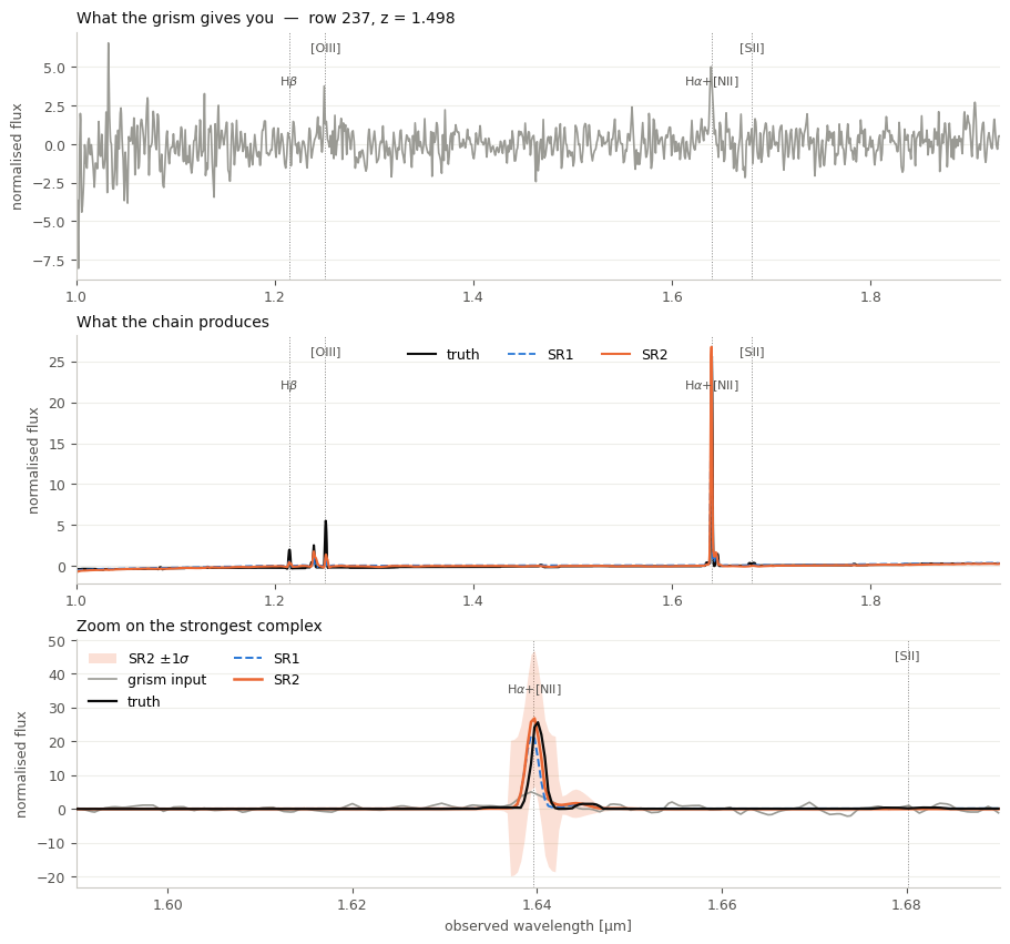
The three panels have different y-scales, on purpose. Each spectrum is normalised by its own mean and standard deviation, and the input’s standard deviation is set by its noise while the target’s is set by its continuum. So a line that is a modest bump in panel 1 is a tall spike in panel 2 even though nothing was added — putting them on one axis would imply a calibration between them that does not exist.

Read panel 3. SR1 (blue) is deliberately cautious and under-shoots the amplitude; SR2 (orange) sharpens it toward the truth. The shaded band is SR2’s own per-pixel uncertainty, and it is wide here — the model is telling you it knows the line is there but not exactly how bright. That is the intended behaviour: the alternative is a confident wrong amplitude.

What neither stage does is add lines elsewhere in the band. That restraint is the whole design, and section 6 is where it gets measured.

4. The redshift is a PDF, not a number

Redshift from a grism is a line-identification problem. A single observed line is consistent with Hα, [O III], [O II] or Lyα, and a model that returns one number has to average between those alternatives — which is how you get a confidently wrong answer. Two earlier designs of this head did exactly that, and both sat at a ~40 % catastrophic floor.

The ZHead returns a distribution over a grid instead. out.z is its mode; out.pz is the whole thing. Keep the PDF.

def top_modes(result, n=3):
    # The package's own mode finder -- the same hypotheses SR2 is run on.
    # It suppresses +/-15 grid bins around each pick, so the modes are distinct
    # line-alias candidates rather than adjacent bins of one peak, and weights
    # each by the probability *mass* in its window rather than by a bin height.
    zs, ws = topk_modes(torch.tensor(result.pz)[None, :],
                        torch.tensor(result.z_grid), n)
    return list(zip(zs[0].tolist(), ws[0].tolist()))


def plot_pz(result, truth, title):
    fig, ax = plt.subplots(figsize=(9, 3.6), constrained_layout=True)
    ax.fill_between(result.z_grid, result.pz, color=SR1_BLUE, alpha=0.30, lw=0)
    ax.plot(result.z_grid, result.pz, color=SR1_BLUE, lw=1.6, label="P(z)")
    ax.axvline(truth, color=INK, lw=1.4, ls="--", label="true redshift")
    # Stagger the mode labels by rank with a leader line: adjacent aliases sit
    # close enough in z that centred labels would overlap.
    for rank, (zm, mass) in enumerate(top_modes(result), start=1):
        height = result.pz[np.argmin(np.abs(result.z_grid - zm))]
        ax.plot([zm], [height], marker="o", ms=5, color=SR1_BLUE, zorder=3)
        ax.annotate(f"mode {rank} · {mass:.0%}", xy=(zm, height),
                    xytext=(zm, 1.05 - 0.09 * rank),
                    textcoords=("data", "axes fraction"), ha="center",
                    fontsize=8, color=MUTED,
                    arrowprops=dict(arrowstyle="-", lw=0.7, color="#c9c8c2"))
    ax.set_xlim(0, 2.6)
    ax.set_ylim(0, result.pz.max() * 1.5)     # headroom for the mode labels
    ax.set_xlabel("redshift")
    ax.set_ylabel("probability")
    ax.set_title(title, color=INK, loc="left")
    ax.legend(loc="upper right")
    ax.grid(axis="y", alpha=0.7)
    ax.set_axisbelow(True)
    plt.show()


for rank, (zm, mass) in enumerate(top_modes(out), start=1):
    print(f"mode {rank}:  z = {zm:.3f}   mass = {mass:.3f}")
print(f"\ntrue z = {z_true[i]:.3f}")

plot_pz(out, z_true[i], f"row {i}: unambiguous — one mode holds nearly all the mass")

mode 1:  z = 1.510   mass = 1.000
mode 2:  z = 1.427   mass = 0.000
mode 3:  z = 0.491   mass = 0.000

true z = 1.498

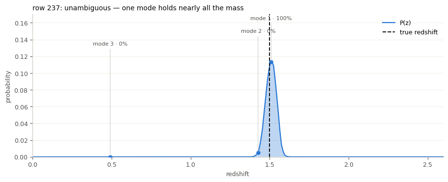
That galaxy is the easy case: one mode carries almost all the probability mass, it sits on the truth, and z_err is correspondingly small. The two remaining modes are the leftovers after suppression — real but negligible.

Section 5 finds the interesting case.

5. Photometry, and why it must be noisy

Three broadband colours break most of the alias degeneracy, which is the entire reason the redshift head takes photometry at all. But the catalogue photometry in this dataset is noiseless truth, and a metric measured on noiseless truth photometry is not a metric. apply_phot_noise adds the same 0.05 mag jitter the head was trained with.

We run the whole subset three ways: with realistic photometry, with the noiseless catalogue values, and with none.

gen = torch.Generator().manual_seed(0)         # seeded, so the run reproduces
phot_noisy = apply_phot_noise(torch.tensor(phot_true, dtype=torch.float32),
                              0.05, gen).numpy()


def run_chain(phot, batch=64):
    results = []
    for s in range(0, len(flux_low), batch):
        p = None if phot is None else phot[s:s + batch]
        results += pipe.predict(flux_low[s:s + batch],
                                flux_low_err[s:s + batch], phot=p)
    return results


outs = run_chain(phot_noisy)
outs_clean = run_chain(phot_true)
outs_nophot = run_chain(None)
print(f"{len(outs)} spectra through the chain, three ways")

512 spectra through the chain, three ways

configs = {
    "grism + Roman imaging, 0.05 mag noise": outs,
    "grism + noiseless catalogue photometry": outs_clean,
    "grism only (photometry mean-imputed)": outs_nophot,
}

print(f"{'configuration':40s} {'NMAD':>8s} {'med |dz|':>9s} {'catastrophic':>13s}")
for label, res in configs.items():
    m = redshift_summary(np.array([r.z for r in res]), z_true)
    print(f"{label:40s} {m['nmad']:8.4f} {m['median_abs_dz']:9.4f} "
          f"{m['catastrophic_frac']:12.1%}")

configuration                                NMAD  med |dz|  catastrophic
grism + Roman imaging, 0.05 mag noise      0.0068    0.0046         6.1%
grism + noiseless catalogue photometry     0.0064    0.0046         4.7%
grism only (photometry mean-imputed)       0.0219    0.0152        27.5%

The first row is the deployable configuration, and it lands on the published numbers (NMAD 0.0065 and 5.1 % catastrophic on the full 7,334-row test split; this is a 512-row draw from it, so expect a little scatter).

Two cautions on the other two rows.

The noiseless row is barely better than the noisy one. That is the point of restricting to three bands: three broadband colours are not a complete SED, so there is very little for the head to cheat with. Hand a redshift head a catalogue’s every filter with no noise and it stops needing the spectrum at all, and the score stops describing the instrument.

phot=None is not a grism-only model. The head was trained with photometry, so passing None feeds it its training-mean colours: an out-of-distribution input, not a clean ablation of the information. Read that row as “the colour prior is carrying most of the redshift accuracy”, not as a measurement of the grism-only information floor. That floor is set by physics — with one line in band the identification is genuinely alias-degenerate — and pinning it down would take a head trained without colours, which is a separate experiment.

fig, axes = plt.subplots(1, 2, figsize=(9, 4.4), constrained_layout=True,
                         sharex=True, sharey=True)
zline = np.linspace(0, 2.6, 200)

for ax, (label, res, colour) in zip(axes, [
        ("grism + Roman imaging (deployable)", outs, SR1_BLUE),
        ("photometry mean-imputed", outs_nophot, SR2_ORANGE)]):
    zp_i = np.array([r.z for r in res])
    frac = np.mean(np.abs(zp_i - z_true) / (1 + z_true) > 0.15)
    ax.fill_between(zline, zline - 0.15 * (1 + zline), zline + 0.15 * (1 + zline),
                    color="#e8e7e2", lw=0, zorder=0)
    ax.plot(zline, zline, color=INK, lw=1.0, zorder=1)
    ax.scatter(z_true, zp_i, s=9, color=colour, alpha=0.55, lw=0, zorder=2)
    ax.set_title(f"{label}\n{frac:.1%} catastrophic", color=INK, loc="left")
    ax.set_xlabel("true redshift")
    ax.set_xlim(0, 2.6)
    ax.set_ylim(0, 2.6)
    ax.grid(alpha=0.7)
    ax.set_axisbelow(True)

axes[0].set_ylabel("predicted redshift")
plt.show()

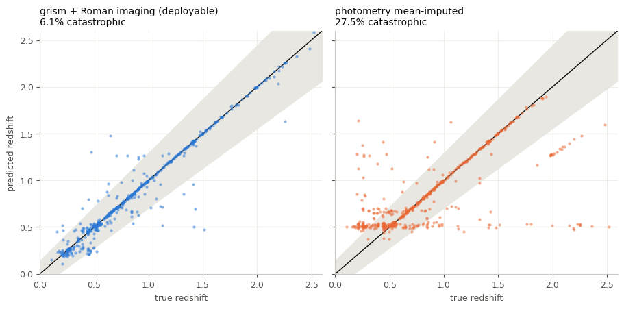
The shaded corridor is the ±0.15 catastrophic boundary, and the two panels fail in visibly different ways.

On the left the failures are not scattered noise: they cluster at particular (true, predicted) pairs — systematic line misidentifications, each cluster one alias. On the right a horizontal track appears, where the head, deprived of colour, falls back on its prior and returns nearly the same redshift regardless of the input. Both are structure a point estimate hides and a PDF exposes.

When the point estimate is wrong

Below we take one of those catastrophic outliers and ask what its PDF was actually saying.

zp = np.array([r.z for r in outs])
bad = np.where(np.abs(zp - z_true) / (1 + z_true) > 0.15)[0]
print(f"{len(bad)} catastrophic outliers out of {len(zp)}")


def truth_rank(row):
    # Which mode, if any, landed on the true redshift.
    for rank, (zm, _) in enumerate(top_modes(outs[row])):
        if abs(zm - z_true[row]) / (1 + z_true[row]) < 0.05:
            return rank
    return None


# Of the failures whose *second* mode is the right answer, show the one where
# that runner-up carries the most mass -- the clearest instance of the pattern.
runners_up = [r for r in bad if truth_rank(r) == 1]
k = max(runners_up, key=lambda r: top_modes(outs[r])[1][1])
modes = top_modes(outs[k])

print(f"{len(runners_up)} of them have the truth as their second mode\n")
print(f"row {k}:  true z = {z_true[k]:.3f},  point estimate = {zp[k]:.3f} "
      f"(z_err = {outs[k].z_err:.3f})")
for rank, (zm, mass) in enumerate(modes, start=1):
    flag = ("  <- the truth"
            if abs(zm - z_true[k]) / (1 + z_true[k]) < 0.05 else "")
    print(f"  mode {rank}:  z = {zm:.3f}   mass = {mass:.3f}{flag}")

plot_pz(outs[k], z_true[k],
        f"row {k}: the point estimate is wrong, the PDF is not")

31 catastrophic outliers out of 512
18 of them have the truth as their second mode

row 302:  true z = 0.904,  point estimate = 1.230 (z_err = 0.201)
  mode 1:  z = 1.230   mass = 0.456
  mode 2:  z = 0.841   mass = 0.483  <- the truth
  mode 3:  z = 0.968   mass = 0.038  <- the truth

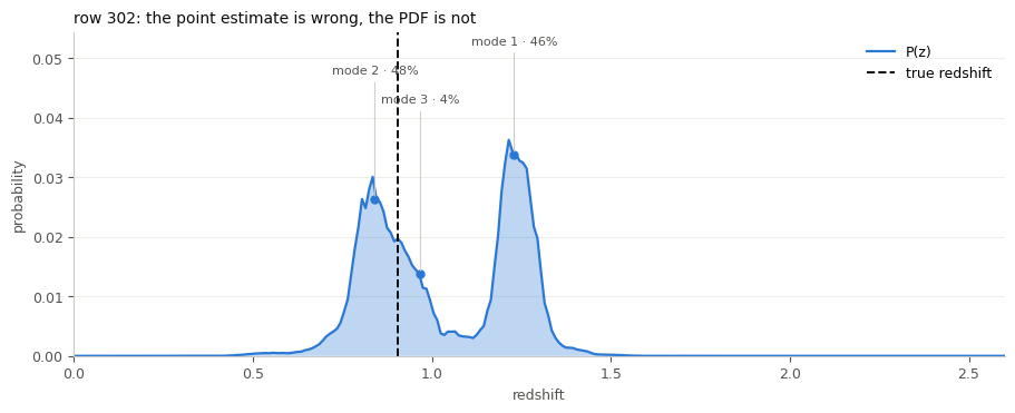
This is why out.pz is worth keeping. The point estimate is the tallest bin, but the runner-up mode carries more probability mass than it does: the model is not confidently wrong here, it is genuinely split between two readings of the same line, and z_err is wide because of it.

A pipeline that propagates the PDF can act on that — deprioritise the source, or carry both hypotheses forward. One that stores only z cannot tell this source apart from a confident, narrow, correct one.

SR2 uses the same information: it runs once per redshift hypothesis and combines by mode mass, so when the top mode is wrong the right lines still get drawn, at reduced weight.

6. Line recovery, split by recoverability

Here is the metric that matters, and the reason it is shaped the way it is.

A single averaged “how much line flux did you recover” number can be improved two ways: by getting better, or by hallucinating harder. Those are opposite behaviours, and no average distinguishes them. So the score is binned by whether the line was recoverable from the low-resolution data at all, using the per-line integrated S/N labels loaded in section 3:

bin	integrated line S/N	what it tests
unrecoverable	< 1	the control — a good model scores ≈ 0 here
marginal	1 – 3	the hard, interesting regime
good	3 – 6	should be recovered
strong	> 6	should be recovered well

A model scoring 0.85 in strong and 0.85 in unrecoverable would be worthless, and a single averaged metric would call it the better model. Read the first row first.

truth_all = np.stack([ds[j][1].numpy() for j in range(len(ds))])
sr1_all = np.stack([to_model_space(r.flux_sr1, flux_low[j])
                    for j, r in enumerate(outs)])
sr2_all = np.stack([to_model_space(r.flux_sr, flux_low[j])
                    for j, r in enumerate(outs)])

rec = {stage: line_amplitude_recovery(pred, truth_all, ds.line_snr.numpy())
       for stage, pred in (("SR1", sr1_all), ("SR2", sr2_all))}

bins = list(rec["SR1"])
print(f"{'recoverability':16s} {'n':>5s} {'SR1':>8s} {'SR2':>8s}")
for b in bins:
    print(f"{b:16s} {rec['SR1'][b]['n']:5d} "
          f"{rec['SR1'][b]['median']:8.2f} {rec['SR2'][b]['median']:8.2f}")

recoverability       n      SR1      SR2
unrecoverable       71    -0.04     0.00
marginal           154     0.13     0.44
good                58     0.65     0.82
strong              30     0.63     0.75

fig, ax = plt.subplots(figsize=(7.4, 4.2), constrained_layout=True)
x = np.arange(len(bins))
w = 0.36

for off, stage, colour in ((-w / 2 - 0.01, "SR1", SR1_BLUE),
                           (w / 2 + 0.01, "SR2", SR2_ORANGE)):
    vals = [rec[stage][b]["median"] for b in bins]
    ax.bar(x + off, vals, w, color=colour, label=stage, zorder=2)
    for xi, v in zip(x + off, vals):
        ax.annotate(f"{v:.2f}", (xi, v), textcoords="offset points",
                    xytext=(0, 4 if v >= 0 else -12), ha="center",
                    fontsize=8, color=MUTED)

ax.axhline(1.0, color=INK, lw=1.0, ls="--", zorder=1)
ax.annotate("true amplitude", (len(bins) - 0.45, 1.0),
            textcoords="offset points", xytext=(0, 4), ha="right",
            fontsize=8, color=MUTED)
ax.axhline(0, color="#c9c8c2", lw=0.8, zorder=1)
ax.set_ylim(top=1.28)
ax.set_xticks(x)
ax.set_xticklabels([f"{b}\n(n = {rec['SR1'][b]['n']})" for b in bins])
ax.set_ylabel("median recovered flux fraction")
ax.set_title("Line amplitude recovery, binned by what the data could show",
             color=INK, loc="left")
ax.legend(loc="upper left")
ax.grid(axis="y", alpha=0.7)
ax.set_axisbelow(True)
plt.show()

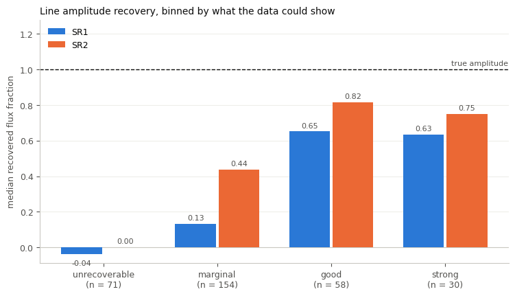
This reproduces the published pattern on a 512-row draw. SR2 sharpens recoverable lines substantially toward truth — and leaves the undetectable ones at essentially zero. The leftmost pair is the one to check on any model you train yourself: a bar that climbs there is a model inventing lines, however good the rightmost pair looks.

SR1’s unrecoverable bar sits slightly below zero. That is a conservative model declining to draw, not an error.

Per-line presence probabilities

SR2 also emits a presence probability for each of its 98 rest-frame features. For the example galaxy from section 3:

rest_aa = dict(LINE_LIST_REST_AA)

print(f"{'feature':22s} {'p':>5s}   observed")
for j in np.argsort(out.presence)[::-1][:8]:
    name = out.line_names[j]
    lam_obs = rest_aa[name] * (1 + z_true[i])
    where = (f"{lam_obs * 1e-4:.3f} µm" if 10000 < lam_obs < 19300
             else "out of band")
    print(f"{name:22s} {out.presence[j]:5.2f}   {where}")

feature                    p   observed
[NII]_6548              0.93   1.636 µm
Halpha_6563             0.89   1.640 µm
[OIII]_5007             0.73   1.251 µm
[OIII]_4959             0.69   1.239 µm
[NII]_6583              0.66   1.645 µm
Hbeta_4861              0.61   1.215 µm
[SIII]_9531             0.23   out of band
[FeII]_16435            0.21   out of band

Features falling outside the grism band are gated off in SR2’s line branch, so a high presence probability there costs nothing and means nothing — read this list together with the observed wavelength.

7. From the command line

Everything above has a CLI equivalent, which is usually what you want for a catalogue rather than for a notebook.

!specsr-roman info

specsr-roman 0.1.0
torch 2.11.0+cu128 | cuda available: False
hub repo: aryana-haghjoo/roman-spectral-superresolution
canonical chain:
  sr1    sr1_ou2024_v6
  zhead  zhead_ou2024_roman_med3_noisy
  sr2    sr2_ou2024_v5_romanonly
  extra [extract]: ok
  extra [train]: ok
  extra [hub]: ok

# run the chain over an npz holding flux_low[, flux_low_err, phot, wavelength_low]
specsr-roman predict spectra.npz --out predictions.npz --phot-tier medium

# reproduce the published metrics and figures from a frozen prediction cache
specsr-roman evaluate cache   --out pred_cache.npz
specsr-roman evaluate metrics --cache pred_cache.npz
specsr-roman evaluate figures --outdir figures/

# the audit that keeps the line-recovery claims honest
specsr-roman evaluate prior

Training each stage is one command and one config file:

specsr-roman train sr1   --config configs/sr1.yaml
specsr-roman train zhead --config configs/zhead.yaml     # needs SR1
specsr-roman train sr2   --config configs/sr2.yaml       # needs SR1 + ZHead

8. Where to go next

• Quickstart — the same API in reference form.

• Data guide — the full dataset, the splitting rule, and the photometric tiers.

• Training guide — including why SR2’s best epoch is 4, which is the design working rather than a truncated run.

• Evaluation guide — the metrics above, plus the prior-dominance audit.

• ARCHITECTURE.md — the full design, the losses, and why each one is shaped the way it is.

Before you use this on anything real

• These results are on a simulation’s manifold. Targets are Diffsky model SEDs with that simulation’s line physics. A model can score well by learning the manifold rather than by measuring anything, and no reconstruction metric distinguishes the two — which is why the package ships a prior-dominance audit. The published SR1 sits at r ≈ 0.45: it reads the data about half as much as it could.

• Trained on simulations, not sky. Real Roman spectra will differ, and domain adaptation is open work.

• The catastrophic rate is physics, not a bug to tune away. With a single line in band the identification is genuinely ambiguous. Photometry breaks most of that degeneracy and cannot break all of it — so propagate the PDF.